sunfluidh:sunfluidh

Table des matières

Overview of key points for using Sunfluidh

Overview of key points for using Sunfluidh

Click here to come back to user's guide contents

Click here to go to the data-set page (input file)

This page summarizes some key points for using the code Sunfluidh in order to better understand the use of Sunfluidh.

Computational domain

The computational domain is the discrete space where equations are solved for flows simulations. It is defined with the namelist “ Domain_Features ”. This namelist contains every data to set up the domain size, the meshsize (the number of cells per direction) and the grid type (regular or not regular). If the grid is regular, every cells have the same size along a given direction. In this case, Sunfluidh builds directly the grid. If the grid is non regular, you should generate speficic files with the mesh generator MESHGEN. These specific files are read by Sunfluidh at the beginning of the computation.

Staggered grid

The spatial discretization of equations is carried out on a staggered grid :

The velocity components are located at the cell-faces
The scalar quantities (temperature, pressure, density, …) are located at the center of cells.

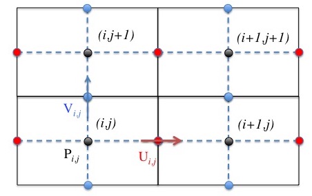
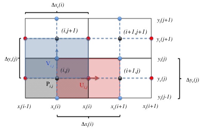
Scalar quantities and velocity components are therefore their own coordinate set as this can be seen on this 2D sketch (same rules are adopted for a 3D configuration). Coordinate sets are defined from cell-centre coordinates {$x_c(i), y_c(j)$} and cell-face coordinates {$x_i(i), y_i(j)$}:
- for any scalar quantity like the pressure $P(i,j)$ : {$x_c(i),y_c(j)$}
- for the horizontal velocity component $U(i,j)$ : {$x_i(i),y_c(j)$}
- for the vertical velocity component $V(i,j)$ : {$x_c(i),y_i(j)$}

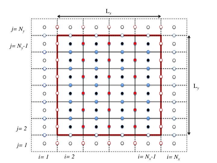
Ghost-cells

The code uses ghost-cells at the domain's ends in order to handle the boundary conditions. These ghost-cells are placed around the computational domain, which is plotted with red lines in the next figure.

The grid size over the computational domain, which is set in the input data file, is enhanced by two in each direction (for example, a 2D grid size $64 \times 64$ over the computational domain becomes $66 \times 66$ in the code).

Boundary conditions

This part is particularly delicate. Please, spend time to read the three sub-sections just below about the boundary conditions and pay attention to the different examples proposed.

At the domain's ends

By default, the computational domain is an enclosed cavity : the domain ends are walls. New boundary conditions can be defined in the data file in place of the default ones by means of the namelists :

Inlet_Boundary_Conditions for inflow features
Outlet_Boundary_Conditions for outflow features
Border_Domain_Boundary_Conditions for periodic conditions or symmetry conditions.

The inlet/outlet boundary conditions overwrite the default wall conditions only on areas defined by the user. Domain ends can be therefore defined from several types of boundary conditions (inlet/wall, outlet/wall, … see here for some examples.
The “border” boundary conditions overwrite the whole specified domain end.

See here for a concrete example showing how to build a boundary condition set up at the domain's ends.

Wall boundary conditions can be specified for different physical quantities with the following namelist :

for velocity : Velocity_Wall_Boundary_Condition_Setup
for temperature : Heat_Wall_Boundary_Condition_Setup
for pressure, the wall boundary condition is always the null normal derivative.

If you do not specify any wall boundary conditions or “border” boundary conditions in the input data file, Sunfluidh assumes default boundary conditions which are :

for velocity : the usual no-slip conditions for tangential velocity components and the impermeability condition for the normal component.
for temperature : Adiabatic condition (zero heat flux)

Immersed bodies

Immersed bodies can be placed in the computational domain in order to build more complex flow geometries. Several geometries are available :

Polyhedrons (see the namelist Polyhedral_Immersed_Bodies)
Cylinders (see the namelist Cylindrical_Immersed_Bodies)

These data setup can be used in 2D and 3D configurations.

When walls of bodies are aligned with the cartesian grid (e.g. for rectangle or cube), you must pay attention to the cell faces match the walls in order to ensure a perfect accuracy on the location of the body.

Linking wall boundary conditions with immersed bodies and walls of the domain ends

You can build different sets of wall boundary conditions for the velocity components and temperature from the namelists previously named (Velocity_Wall_Boundary_Condition_Setup, Heat_Wall_Boundary_Condition_Setup). Each set must be tagged by means of the indentifier “Wall_BC_DataSetName”:

The 1st set is identified with Wall_BC_DataSetName=“Set1” (for velocity and temperature)
The 2nd set is identified with Wall_BC_DataSetName=“Set2” (for velocity and temperature)
and so on …

The namelists of immersed bodies also get an indentifier “Wall_BC_DataSetName” which can be named with the tag corresponding to the appropriate wall boundary conditions.

By default, the wall boundary condition “Set1” is always applied at the walls placed at the domain ends (if they exists).
The wall boundary condition “Set1” can be also used for a immersed body.
A set of wall boundary conditions can be used for several immersed bodies

For a better understanding on the boundary conditions, an example is provided here that belongs to the tutorial Tutorial : How to build the input data file

Fluid properties

The fluid properties are defined with the namelist Fluid_Properties .
It is not mandatory to set up all the data of the namelist. Only the data of interest must be considered, the other ones can be ignored.

By default the fluid is incompressible.

You find here some examples :
For an incompressible fluid without heat transfer

 &Fluid_Properties  Reference_Density= 1.0 , Reference_Dynamic_Viscosity = 3.D-03 /

For an incompressible fluid with heat transfer

 &Fluid_Properties  Heat_Transfer_Flow = .true.     ,  Reference_Density= 1.0,
                    Reference_Temperature= 1.0      ,  Reference_Dynamic_Viscosity= 0.71D-02  ,
                    Reference_Heat_Capacity= 1.0.   ,
                    Prandtl = 0.71                  ,  Thermal_Expansion_Coefficient= 1.0 /

For problems with heat transfer, the heat capacity is supposed uniform and constant (except for multi-species flows, it can depend on temperature and species mass fractions).
The thermal diffusivity is computed by the code from the reference values of density, dynamic viscosity and Prandtl number : $\kappa_0= \frac{\mu_0}{\rho_0 Pr}$.
The thermal conductivity is computed by the code from the reference values of heat capacity, dynamic viscosity and Prandtl number : $\lambda_0= \frac{\mu_0.Cp_0}{Pr}$.
The temperature dependance of the dynamic viscosity, thermal diffusivity and thermal conductivity can be taken into account with the Sutherland's law (add the variable Sutherland_Law_Enabled=.true.)
$\mu= \mu_0(T_0).S(T)$ ; $\kappa= \kappa_0(T_0).S(T)$ ; $\lambda= \lambda_0(T_0).S(T)$
where $T_0$ is the reference value of the temperature (Reference_Temperature)
The Sutherland's law reads: $$S(T)=\frac{T^{1.5}.C_1}{T+C_2}$$
where $C_1$ and $C_2$ are parameters which depend on reference pressure (the atmospheric pressure) and reference temperature ($T_0$).
The data “Thermal_Expansion_Coefficient” is related to the buoyancy effect which is activated with the namelist “ Gravity ”. Please, read attentively the documentation related to the gravitational force ( Gravity ) because the data setting depends on the problem treated.

Field's initialization procedure

The initialization procedure relies on specific namelists :

For the velocity components : Velocity_Initialization
For the temperature : Temperature_Initialization
For the species mass fractions (only for multi-species flows) Species_Initialization
For incompressible and immiscible two-phase fluid flows : Two_Fluids_Initialization

These namelists propose several ways for initializing the fields of velocity, temperature, species mass fractions, etc …

The initial density field is generally uniform except for the two-phase flows and sometimes for the multi-species flows.

Numerical time step

The data set up that refers to the time step is in the namelist Simulation_Management. Two ways are possible :

The time step value is imposed by the user ( TimeStep_Type = 0, TimeStep_Max= value).
In this case, the user must set up the time step in such a way the time stability criteria is satisfied (CFL condition). The computation is more accurate as the time step is regular during the time iterations.
The time step value is automatically estimated by the code from the CFL value set by the user (TimeStep_type= 1, CFL_max= value).
The CFL value should be smaller than or equal to 0.5 to ensure the numerical stability of the computation (the value could be depend on the problem).
The time step estimated from the CFL condition is however limited by a maximum value provided by “TimeStep_Max”. Some numerical simulations can start with a fluid at rest or with very small velocity values. As a consequence, the time step calculated from the CFL condition is irrelevant.

When the user wants to acquire results with an accurate time recording rate, he should use an imposed time step. When the user wants to record time series from probes in order perform FFT, it is also strongly advised to use an imposed time step.

Results

Sunfluidh can provides various results of simulation :

Instantaneous fields of physical quantities
statistical fields
time series related to probes

Information on these results is provided on the page "Sunfluidh output files".

Stopping criteria

Three possibilities exist for stopping the simulation by means of data present in the namelist Simulation_Management :

Final_Time : The simulation stops when this time is reached.
Temporal_Iterations_Number : The simulation stops when this number of time-step iterations is reached.
Steady_Flow_Stopping_Criterion_Enabled , Steady_Flow_Stopping_Criterion :When the first parameter is set to “.True.”, the simulation stops when the residu value (based on the L2-norm of the time-derivatives of physical quantities, see the part “checking files” in "Sunfluidh output files" ) becomes smaller than the value of “Steady_Flow_Stopping_Criterion”. This way is only relevant for the computation of steady flows.

The first criterion statisfied among the three ones stops the simulation.