Ceci est une ancienne révision du document !
Table des matières
Tutorial : How to build the input data file ?
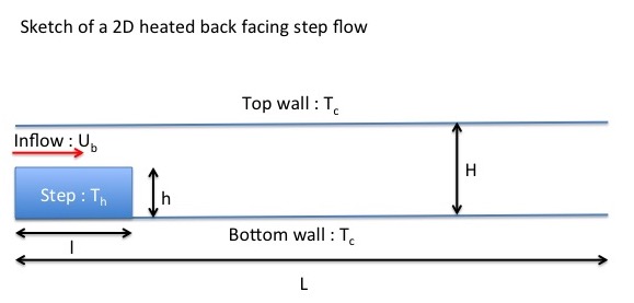
This tutorial shows how to create an input data file for a 2D heated back-facing step flow.
After providing the main features of the problem, explanations on how to build step by step the corresponding data file is shown.
Each relevant namelist is commented and referred to other pages for more details.
The user can create its own data file by resorting to any highlighted data set.
Flow features
Description
The computation is on a 2D heated back-facing step flow. The temperature of the bottom and top walls is imposed to $T_c$ and the temperature of the step walls is $T_h$. The inflow is fixed with an uniform velocity profile $U_b$ at temperature $Tc$. We consider an incompressible flow under the Boussinesq hypothesis : the physical properties are constant and the thermal buoyancy effect is modelised by the Boussinesq hypothesis : $F_b= -\rho_0.\beta.g_0.(T - T_0)$ (see the page Gravity for more details). We suppose the fluid as a perfect gas. As a consequence, $\beta= \frac{1}{T_0}$
Dimensionless data
Reference scales for the dimensionless problem :
- the fluid density $\rho_0$
- the bulk velocity $U_b$
- the kinematic viscosity $\mu_0$
- the step height
- the temperature $T_c$
From the previous reference scales, we define the Reynolds number : $Re_h= \frac{\rho_0 \dot U_b \dot h}{\mu_0}$ and the dimensionless temperature $T*= \frac{T}{T_c}$.
We therefore deduce the following dimensionless data :
- Fluid density $\rho_0*=1$
- Inflow bulk velocity $U_b*= 1$
- Bottom and top wall temperature $T_c*=1$
- Thermal expansion coefficient $\beta*=1$
- Step height $h*= 1$
Any other data of the problem are set to :
- Domain length : $L*=12$
- Domain height : $H*= 2$
- Step length : $l*= 2$
- Reynolds number $Re_h= 100$
- Step wall temperature $T_h*= 2$
- Gravity constant $g*= \frac{g_0 \dot h}{U_b^2}= 1$
- Prandtl number $Pr= 0.71$
Data setup
We now build the data file by selecting the relevant namelists in the lookup list. We only keep the relevant variables (that must be explicitly set). The others ones are removed. We need to set :
The physical properties for an incompressible fluid without multi-species components
We report here the dimensionless data set about the fluid properties defined above.
  &Fluid_Properties  Variable_Density            = .false. , !---- Incompressible fluid
                     Constant_Mass_Flow          = .true.  , !---- The mass flowrate is constant
                     Heat_Transfer_Flow          = .true.  , !---- Heat transfer enabled
                     Reference_Density            = 1.0    , !---- Dimensionless fluid density
                     Reference_Dynamic_Viscosity  = 1.D-02 , !---- Dimensionless dynamic viscosity (=1/Reh)
                     Reference_Temperature        = 1.0    , !---- Dimensionless reference temperature (=Tc*)
                     Prandtl                      = 0.71   , !---- Prandtl number value
                     Thermal_Expansion_Coefficient= 1.0   /  !---- Dimensionless thermal expansion coeffficient
For more examples about the fluid properties setting click here.
Initialization of the velocity, temperature and density over the domain
The fluid density is implicitly initialized with a uniform field because the fluid is incompressible and homogeneous. No data set is therefore required.
The initial fluid temperature is uniform over the domain.
 &Temperature_Initialization Temperature_Reference_Value          = 1.0 ,  !--- Default value
                             Initial_Field_Option_For_Temperature = 0   /  !--- Initialization of the field with the default value
The initial velocity field is defined by spreading out the inflow velocity profile. This choice allows us to ensure a perfect flowrate conservation between inflow and outflow for the first time step.
  &Velocity_Initialization  I_Velocity_Reference_Value = 0.0     ,  !--- default value for the I-velocity component
                            J_Velocity_Reference_Value = 0.0     ,  !--- default value for the J-velocity component
                            K_Velocity_Reference_Value = 0.0     ,  !--- default value for the K-velocity component
                          Initial_Field_Option_For_Velocity_I = 3 , !--- the inflow velocity profile is spread out in the I-direction
                          Initial_Field_Option_For_Velocity_J = 0 , !--- Initialization of the field with the default value
                          Initial_Field_Option_For_Velocity_K = 0. /!--- Initialization of the field with the default value
The velocity field initialization depends on the velocity profile defined in the namelist Inlet_Boundary_Condition.
For more examples about the velocity field initialization click here.
Forces applied to the fluid
Only the gravity is considered through the thermal buoyancy effect. The gravity force is oriented facing downward.
 &Gravity Gravity_Enabled= .true.          ,     !--- the gravity force is enabled
          Gravity_Angle_IJ= 0.0            ,     !--- {IJ} angle (in degree unit)
          Gravity_Angle_IK= 90.0           ,     !--- {IK} angle (in degree unit)
          Reference_Gravity_Constant= 1.D+00/    !--- dimensionless value of g0
Domain configuration
We here suppose a regular cartesian grid. We set the geometrical configuration, the place and the size of the domain as well as the mesh size.
For a sequential computing
  &Domain_Features Geometric_Layout               = 0,         !--- Option value for a cartesian geometry
                   Start_Coordinate_I_Direction   = 0.0  ,     !--- Start coordinate along the I-direction
                   End_Coordinate_I_Direction     = 12.  ,     !--- End coordinate along the I-direction
                   Start_Coordinate_J_Direction   = 0.0  ,     !--- Start coordinate along the J-direction
                   End_Coordinate_J_Direction     = 2.0  ,     !--- End coordinate along the J-direction
                   Start_Coordinate_K_Direction   = 0.00 ,     !--- Start coordinate along the K-direction
                   End_Coordinate_K_Direction     = 0.00 ,     !--- End of the domain along the K-direction
                   Cells_Number_I_Direction       = 384 ,      !--- Number of cells along the I-direction (not counting the ghost cells)
                   Cells_Number_J_Direction       = 128 ,      !--- Number of cells along the J-direction (not counting the ghost cells)
                   Cells_Number_K_Direction       = 1,         !--- Number of cells along the K-direction (not counting the ghost cells)
                   Regular_Mesh                   = .true. /   !--- The grid is regular for any direction
For OpenMP or MPI parallel computing
(Not for the release SUNFLUIDH_EDU).
The code SUNFLUIDH can perform OpenMP or MPI computing (if it has been compiled with the appropriate options, see How to configure the makefile).
The user can configure a parallel computing from the data file by setting the appropriate variables of the previous namelist. All details for our example are given here.
Boundary conditions
The problem gets different type of boundary conditions :
- For the velocity :
- Common wall boundary conditions : No slip and impermeable boundary conditions
- Inflow boundary condition : uniform velocity profile imposed.
- Outflow boundary condition : mass flowrate conservation
- For the heat transfer :
- Wall boundary conditions : Temperature imposed
- Inflow boundary condition : Temperature imposed
- Outflow boundary condition : zero temperature gradient
Wall boundary conditions
The walls are associated with two different immersed bodies:
- the domain ends which gets the top and bottom walls
- the step
The wall boundary conditions for the velocity are identical for every walls of the domain and they correspond to the wall boundary conditions stated by default in the code SUNFLUIH. As a consequence, they need not to be explicitly declared.
The wall temperature are however different according to the immersed bodies cited above ($T_c*=1$ for the bottom and the top walls, $T_h*=2$ for the step walls). We must define two sets of boundary conditions for the temperature.
Set 1 (for the walls of domain ends) : Only the data associated to the top (front) and bottom (back) walls are present, the other ones are useless as the corresponding walls are absent.
 &Heat_Wall_Boundary_Condition_Setup
  Back_Heat_BC_Option     = 0    , Front_Heat_BC_Option    = 0 ,    !--- option value for  temperature imposed
  Back_Heat_Function_Type = 0    , Front_Heat_Function_Type= 0 ,    !--- option value for defining a uniform value of T over the wall
  Back_Wall_BC_Value      = 1.0  , Front_Wall_BC_Value     = 1.0 /  !--- temperature value (here Tc)
Set 2 (for the walls of the step)_ : Only the data associated to the top (noted back for immersed bodies) and right (noted west for immersed bodies) walls are present, the other ones are useless as the corresponding walls have no role in the current problem.
 &Heat_Wall_Boundary_Condition_Setup
  Back_Heat_BC_Option     = 0    , East_Heat_BC_Option    = 0 ,    !--- option value for  temperature imposed
  Back_Heat_Function_Type = 0    , East_Heat_Function_Type= 0 ,    !--- option value for defining a uniform value of T over the wall
  Back_Wall_BC_Value      = 2.0  , East_Wall_BC_Value     = 2.0 /  !--- temperature value (here Tc)
We must now build the immersed bodies.
On the walls of the domain ends :
This is already made. Keep in mind that the computational domain is enclosed by default. Walls are automatically placed at the domain ends by the code except when other boundary conditions are specified by the user (which are going to replace the walls).
For building the step :
 &Polyhedral_Immersed_Bodies
                         Xi_1= 0.0  , Xj_1= 0.0  ,Xk_1= 0.0 , !--- Coordinates of the 1st corner
                         Xi_2= 2.0  , Xj_2= 0.0  ,Xk_2= 0.0 , !--- Coordinates of the 2nd corner
                         Xi_3= 2.0  , Xj_3= 1.0  ,Xk_3= 0.0 , !--- Coordinates of the 3rd corner
                         Xi_4= 0.0  , Xj_4= 1.0  ,Xk_4= 0.0 , !--- Coordinates of the 4th corner
                         Identifier_Value= 2,                 !--- ID value associated to the suitable set of wall boundary conditions
- By default, the first set of wall boundary conditions is always associated to walls placed at the domain ends (No ID value is needed)
- For other immersed solid bodies, the ID value links the body walls with the set of wall boundary conditions that gets the same rank order in the data file (here, the 2nd set because Identifier_Value= 2).
- Beware to the rule adopted for naming the walls (East,west,front, back, north,south). They seem inconsistent between walls of domain ends and any other immersed body but it is not the case!
- For more information on the rules of construction Click here
- For more details on the data setup of the wall boundary conditions
- For more details on the data setup for building immersed solid bodies
Inlet boundary conditions
The inflow conditions are uniform profiles of velocity ($U_b=1$) and temperature ($T_c= 1$).
 &Inlet_Boundary_Conditions
              Type_of_BC                     = "INLET",  !--- Specify inflow conditions (mass flowrate and other physical quantities imposed)
              Direction_Normal_Plan          = 1    ,    !--- Normal vector of the inlet plan oriented along the I-direction
              Plan_Location_Coordinate       = 0.0  ,    !--- Position of the inlet along the normal direction
              Start_Coordinate_of_First_Span = 1.0  ,    !--- Start coordinate of the inlet along the direction related to the 1st span (here J-direction, just above the step)
              End_Coordinate_of_First_Span   = 2.0  ,    !--- End coordinate of the inlet along the direction related to the 1st span (here J-direction, at the top wall)
              Start_Coordinate_of_Second_Span= 0.0  ,    !--- Start coordinate of the inlet along the direction related to the 2nd span (here K-direction)
              End_Coordinate_of_Second_Span  = 0.0  ,    !--- End coordinate of the inlet along the direction related to the 1st span (here K-direction)
              Flow_Direction                 = 1    ,    !--- The flow is oriented along the increasing I-index
              Define_Velocity_profile        = 0    ,    !--- Option value for a uniform velocity profile
              Normal_Velocity_Reference_Value= 1.0  ,    !--- Value of the normal velocity-component (here Ub= 1) , the other ones are null.
              Temperature_Reference_Value    = 1.0 /     !--- Value of the temperature (uniform distribution, here Tc= 1)
Outlet boundary conditions
We here select usual outflow boundary conditions based on the flowrate conservation for treating the normal velocity component. The outflow boundary conditions other physical quantities are zero gradient condition.
 &Inlet_Boundary_Conditions
              Type_of_BC                     = "OUTLET", !--- Specify the outflow conditions cited above
              Direction_Normal_Plan          = 1    ,    !--- Normal vector of the inlet plan oriented along the I-direction
              Plan_Location_Coordinate       = 0.0  ,    !--- Position of the inlet along the normal direction
              Start_Coordinate_of_First_Span = 0.0  ,    !--- Start coordinate of the inlet along the direction related to the 1st span (here J-direction, at the floor wall)
              End_Coordinate_of_First_Span   = 2.0  ,    !--- End coordinate of the inlet along the direction related to the 1st span (here J-direction, at the top wall)
              Start_Coordinate_of_Second_Span= 0.0  ,    !--- Start coordinate of the inlet along the direction related to the 2nd span (here K-direction)
              End_Coordinate_of_Second_Span  = 0.0  ,    !--- End coordinate of the inlet along the direction related to the 1st span (here K-direction)
              Flow_Direction                 = 1    /    !--- The outflow is mainly oriented along the increasing I-index
Border boundary condition
The boundary conditions related to our example are already specified (walls, inflow, outflow conditions). No more boundary conditions must be defined. The namelist “Border_Domain_Boundary_Conditions” is therfore set as :
  &Border_Domain_Boundary_Conditions
        West_Border= 0  ,              !--- Boundary conditions already defined for the left end of the domain (corresponding to the lower I-index)
        East_Border= 0  ,              !--- Boundary conditions already defined for the right end of the domain (corresponding to the upper I-index)
        Back_Border= 0  ,              !--- Boundary conditions already defined for the bottom end of the domain (corresponding to the lower J-index)
        Front_Border= 0 /              !--- Boundary conditions already defined for the top end of the domain (corresponding to the upper J-index)
Numerical Methods
We remind the user the equations are solved with a projection method. The numerical methods used in the code SUNFLUIDH are commented in the documents for the full version or documents for the educative version.
For solving the conservation equations for velocity and temperature, we choose a 2nd order scheme in space and time.
- The spatial discretization for the convective flux is a 2nd order centered scheme (conservative form)
- The spatial discretization for the viscous/conductive terms is also a 2nd order centered scheme (this way is imposed, no choice is possible)
- The time discretization is a 2nd order Backward Differentiation Formula (semi-implicit method build on the viscous/conductive terms)
The Poisson's equation is solved a Successive Over-Relaxation method coupled with a nV-cycle multigrid method for accelerating the convergence. As the flow is incompressible, a solver version with constant coefficient matrix can be selected.
The data setup is made with the following namelists :
  &Numerical_Methods  NS_NumericalMethod= "BDF2-SchemeO2"                    ,  !--- BDF2 + 2nd order centered scheme
                      MomentumConvection_Scheme="Centered-O2-Conservative"   ,  !--- conservative form for solving the velocity (momentum) equation
                      TemperatureAdvection_Scheme="Centered-O2-Conservative" ,  !--- conservative form for solving the temperature (enthalpy) equation
                      Poisson_NumericalMethod="Home-Multigrid-ConstantMatrixCoef"  / !--- SOR  + multigrid method (homemade release) for solving the Poisson's equation with constant coefficient matrix
As the used solver is a “homemade” release (directly implemented in the code SUNFLUIDH without invoking any external scientific library), the parameters of the SOR + multigrid method are set in the namelist
   &HomeData_PoissonSolver  SolverName="SOR-Redblack",!--- Successive Over-Relaxation (SOR) method based on the red-black algorithm
                            Relaxation_Coefficient= 1.7 , !--- Relaxation coefficient of the SOR method ( 1 <= Relaxation_Coefficient < 2)
                            Number_max_Grid= 5,       !--- Number of grid levels
                            Number_max_Cycle= 10,     !--- Number of multigrid cycles
                            Number_Iteration= 0,      !--- Maximum number of SOR iterations method applied for any grid level, if 0 (or removed) the 3 next data are considered
                            Number_Iteration_FineToCoarseGrid= 3,  !--- number of SOR iterations applied on any grid level during the restriction step (before the coarsest grid computation)
                            Number_Iteration_CoarseToFineGrid= 15, !--- number of SOR iterations applied on any grid level during the prolongation step (after the Coarsest grid computation)
                            Number_Iteration_CoarsestGrid= 15 ,    !--- number of SOR iterations applied on the coarsest grid
                            Convergence_Criterion= 1.D-08 /        !--- convergence tolerance on the residu of the Poisson's equation
- The maximum number of grid level is conditioned by the cell number of the finnest grid. The grid coarsening consists in dividing by two the cell number along each direction. The minimum number of cells on the coarsest grid is two per direction.
- The relaxation coefficient can improve the convergence efficiency but beware of the numerical instabilities. The choice of the relaxation coefficient depends on the problem. The maximum value are about $1.8$ and the minimum value is $1$.
- The red-black algorithm is able to keep the same solution accuracy in parallel computing regardless of the domain decomposition. It can be seen as the combination of Jacobi and Gauss-Seidel methods. As the consequence, the convergence is less efficient than a pure SOR method (or Over Relaxed Gauss-Seidel method) which doas not preserve the solution accuracy in parallel computing in regard to the domain decomposition.
- It could be useful to set the number of SOR iterations to different values for each part of a V-cycle of the multigrid method in order to reduce the total number of operations. Some numerical experiments are shown that only few SOR iterations could be sufficient during the restriction step. A fine setting of the iteration number can improve the performance of the code.
- Beware of the maximum number of multigrid cycles. more larger is this number more longer is the CPU time consuming if the convergence is too slow. Its maximum value is generally approximately 10. Beyond this value, it could be useful to try something else.
- Do not forget the purpose on solving the Poisson's equation : ensure a divergence-free velocity for incompressible flows or the mass preserving in low Mach number hypothesis. This goal is sometimes reached without solving the Poisson's equation with a too much small convergence tolerance…
Simulation control data set
We here resort to a specific namelist named “Simulation_Management. It is also used in the next section “Data acquisition”. We specify here some parameters in order to define the numerical time step as well as stop criteria and recording rates related to backup and check files. Two examples are given. The first one corresponds to a simulation starting at t= 0 with a variable time step.
 &Simulation_Management Restart_Parameter= 0                             ,!--- Option value for starting the simulation from t=0.
       Steady_Flow_Stopping_Criterion_Enabled = .false. ,!--- Stop criterion for steady flows. When it is enabled, residues between two successive flow fields are computed
       Steady_Flow_Stopping_Criterion = 1.D-20          ,!--- convergence tolerance threshold for a steady flow solution (it works only when the previous parameter is enabled)
       Temporal_Iterations_Number = 10                  ,!--- maximum value of time iterations before stopping the computation
       Final_Time = 3.D+01                              ,!--- Maximum value of time before stopping the computation
       TimeStep_Type = 1 ,                              ,!--- Option value for specifying a variable time-step computed from a CFL criterion
       CFL_Min = 0.05                                   ,!--- Minimum value of the CFL criterion imposed by the user when the simulation starts
       CFL_Max = 0.4                                    ,!--- Maximum value of the CFL criterion imposed by the user after n time iterations (here n= 100, see the next parameter)
       Iterations_For_Timestep_Linear_Progress= 100     ,!--- Number of time iterations over which the CFL criterion increase linearly between CFL_Min and CFL_Max
       Simulation_Backup_Rate                 = 1000    ,!--- Recording rate (in time-iteration units) for generating backup files (save_fld_xxxxx_y.d , save_var_xxxxx_y.d)
       Simulation_Checking_Rate               = 200     /!--- Recording rate (in time-iteration units) for writing some relevant check data in a file checkcalc_xxxxx.d
The second example corresponds to a restart of the previous simulation with a uniform time step.
&Simulation_Management Restart_Parameter= 3             ,!--- Option value for resuming the simulation from the end of a previous computation.
       Steady_Flow_Stopping_Criterion_Enabled = .false. ,!--- Stop criterion for steady flows. When it is enabled, residues between two successive flow fields are computed
       Steady_Flow_Stopping_Criterion = 1.D-20          ,!--- convergence tolerance threshold for a steady flow solution (it works only when the previous parameter is enabled)
       Temporal_Iterations_Number = 1000                ,!--- maximum value of time iterations before stopping the computation
       Final_Time = 6.D+01                              ,!--- Maximum value of time before stopping the computation
       TimeStep_Type = 0 ,                              ,!--- Option value for specifying a constant time-step
       Timestep_Max = 1.e-3,                            ,!--- Value of the time step
       Iterations_For_Timestep_Linear_Progress= 100     ,!--- Number of time iterations over which the CFL criterion increase linearly between CFL_Min and CFL_Max
       Simulation_Backup_Rate                 = 1000    ,!--- Recording rate (in time-iteration units) for generating backup files (save_fld_xxxxx_y.d , save_var_xxxxx_y.d)
       Simulation_Checking_Rate               = 200     /!--- Recording rate (in time-iteration units) for writing some relevant check data in a file checkcalc_xxxxx.d
                         Fields_Recording_Rate = 1.D+00 ,
                         Probe_Recording_Rate                   = 10     ,
                         Start_Time_For_Statistics= 1.D+2               ,
                         Time_Range_Statistic_Calculation = 1.D+00  /
For more information on this data set, click here.
- For semi-implicit schemes proposed here, a maximum CFL-value about 0.5 is generally prescribed for usual computations, but it could be smaller for problems with strong gradients.
- For explicit schemes, the CFL criterion also depends on the viscous/diffusive time scales as well as the space dimension of the problem. As a consequence, the CFL value prescribed is generally between $0.5^{n-1}$ and $0.5^n$, where n is the dimension of the problem.
When the time-step value is constant, the user can verify if the CFL criterion is respected by checking regularly the file checkcalc_xxxxx.d
Output data
Here we show an example of usual data acquisition :
- Instantaneous fields
- Statistical fields
- Time series from probes located at specific positions
The various parameters related to each type of output data are originally splitted by topic in the appropriate namelist. For a sake of clarity, they are directly regrouped for each type of output data as shown here :
For instantaneous fields
 &Field_Recording_Setup         Precision_On_Instantaneous_Fields= 2 /                  !--- option value for writing results in double precision (1 = single precision)
 &Simulation_Management         Fields_Recording_Rate = 1.0D-00 /                       !--- Recording rate (in time unit)
 &Instantaneous_Fields_Listing  Name_of_Field = "U" , Recording_Enabled = .true.  /     !--- Recording of the first velocity component enabled
 &Instantaneous_Fields_Listing  Name_of_Field = "V" , Recording_Enabled = .true.  /     !--- Recording of the second velocity component enabled
 &Instantaneous_Fields_Listing  Name_of_Field = "W" , Recording_Enabled = .false. /     !--- Recording of the Third velocity component disabled
 &Instantaneous_Fields_Listing  Name_of_Field = "T" , Recording_Enabled = .true.  /     !--- Recording Temperature enabled
 &Instantaneous_Fields_Listing  Name_of_Field = "P" , Recording_Enabled = .true.  /     !--- Recording Pressure enabled
For statistical fields
 &Simulation_Management Start_Time_For_Statistics= 1.D+2               ,          !--- Start time for computing the statistical fields
                        Time_Range_Statistic_Calculation = 1.D+00      /          !--- time range over which the statistical field computation is performed.
                                                                                        When it has been covered, the results are recorded and a new statistical computation starts again
 &Field_Recording_Setup      Precision_On_Statistical_Fields= 2 ,                 !--- option value for writing results in double precision (1 = single precision)
                             Time_Statistics_Enabled= .true.    ,                 !--- time statistics  are performed (true) - classical statistics (false)
                             Sample_Rate_For_Statistics= 1      ,                 !--- Sample rate (in time iteration unit)
                             Statistic_Space_Average_Type= "NO_SPACE_AVERAGE" /   !--- option on spatial averaged fields
 &Statistical_Fields_Listing  Name_of_Field = "<U>   " , Recording_Enabled = .true.  /   !---- Averaged I-velocity component
 &Statistical_Fields_Listing  Name_of_Field = "<V>   " , Recording_Enabled = .true.  /   !---- Averaged J-velocity component
 &Statistical_Fields_Listing  Name_of_Field = "<P>   " , Recording_Enabled = .true.  /   !---- Averaged pressure
For time-series from probes
                                                                       U    , V     , W      , T      , P     , RHO
 &Probe_Quantities_Enabled  Temporal_Series_For_Quantity_Enabled(:)= .true. , .true., .false., .false., .true., .false.    /    !--- Selection of physical quantities
 &Simulation_Management Probe_Recording_Rate                       = 10                                                     /   !--- Recording rate (in time-iteration unit)
 &Probe_Location  Xi= 2.0 , Xj= 1.5 , Xk= 0.0 /       !---coordinates of probe 1
 &Probe_Location  Xi= 3.0 , Xj= 1.0 , Xk= 0.0 /       !---coordinates of probe 2
- fr