Tutorial : How to build the input data file ?

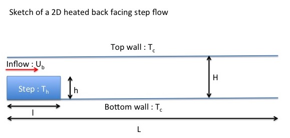
This tutorial shows how to create an input data file for a 2D heated back-facing step flow. After providing the main features of the problem, explanations on how to build step by step the corresponding data file is shown. Each relevant namelist is commented and referred to other pages for more details.
The user can create its own data file by resorting to any highlighted data set.

Flow characteristics

Description

The computation is on a 2D heated back-facing step flow. The temperature of the bottom and top walls is imposed to $T_c$ and the temperature of the step walls is $T_h$. The inflow is fixed with an uniform velocity profile $U_b$ at temperature $Tc$. We consider an incompressible flow under the Boussinesq hypothesis : the physical properties are constant and the thermal buoyancy effect is modelised by the Boussinesq hypothesis : $F_b= -\rho_0.\beta.g_0.(T - T_0)$ (see the page Gravity for more details). We suppose the fluid as a perfect gas. As a consequence, $\beta= \frac{1}{T_0}$

Dimensionless data

Reference scales for the dimensionless problem :

the fluid density $\rho_0$
the bulk velocity $U_b$
the kinematic viscosity $\mu_0$
the step height
the temperature $T_c$

From the previous reference scales, we define the Reynolds number : $Re_h= \frac{\rho_0 \dot U_b \dot h}{\mu_0}$ and the dimensionless temperature $T*= \frac{T}{T_c}$.
We therefore deduce the following dimensionless data :

Fluid density $\rho_0*=1$
Inflow bulk velocity $U_b*= 1$
Bottom and top wall temperature $T_c*=1$
Thermal expansion coefficient $\beta*=1$
Step height $h*= 1$

Any other data of the problem are set to :

Domain length : $L*=12$
Domain height : $H*= 2$
Step length : $l*= 2$
Reynolds number $Re_h= 100$
Step wall temperature $T_h*= 2$
Gravity constant $g*= \frac{g_0 \dot h}{U_b^2}= 1$
Prandtl number $Pr= 0.71$

Data setup

We now build the data file by selecting the relevant namelists in the lookup list. We only keep the relevant variables (that must be explicitly set). The others ones are removed. We need to set :

Simulation control data set

We here resort to a specific namelist named “Simulation_Management. It is also used in the next section “Data acquisition”. We specify here some parameters in order to define the numerical time step as well as stop criteria and recording rates related to backup and check files. Two examples are given. The first one corresponds to a simulation starting at t= 0 with a variable time step.

 &Simulation_Management Restart_Parameter= 0                             ,!--- Option value for starting the simulation from t=0.
       Steady_Flow_Stopping_Criterion_Enabled = .false. ,!--- Stop criterion for steady flows. When it is enabled, residues between two successive flow fields are computed
       Steady_Flow_Stopping_Criterion = 1.D-20          ,!--- convergence tolerance threshold for a steady flow solution (it works only when the previous parameter is enabled)
       Temporal_Iterations_Number = 10                  ,!--- maximum value of time iterations before stopping the computation
       Final_Time = 3.D+01                              ,!--- Maximum value of time before stopping the computation
       TimeStep_Type = 1 ,                              ,!--- Option value for specifying a variable time-step computed from a CFL criterion
       CFL_Min = 0.05                                   ,!--- Minimum value of the CFL criterion imposed by the user when the simulation starts
       CFL_Max = 0.4                                    ,!--- Maximum value of the CFL criterion imposed by the user after n time iterations (here n= 100, see the next parameter)
       Iterations_For_Timestep_Linear_Progress= 100     ,!--- Number of time iterations over which the CFL criterion increase linearly between CFL_Min and CFL_Max
       Simulation_Backup_Rate                 = 1000    ,!--- Recording rate (in time-iteration units) for generating backup files (save_fld_xxxxx_y.d , save_var_xxxxx_y.d)
       Simulation_Checking_Rate               = 200     /!--- Recording rate (in time-iteration units) for writing some relevant check data in a file checkcalc_xxxxx.d

The second example corresponds to a restart of the previous simulation with a uniform time step.

&Simulation_Management Restart_Parameter= 3             ,!--- Option value for resuming the simulation from the end of a previous computation.
       Steady_Flow_Stopping_Criterion_Enabled = .false. ,!--- Stop criterion for steady flows. When it is enabled, residues between two successive flow fields are computed
       Steady_Flow_Stopping_Criterion = 1.D-20          ,!--- convergence tolerance threshold for a steady flow solution (it works only when the previous parameter is enabled)
       Temporal_Iterations_Number = 1000                ,!--- maximum value of time iterations before stopping the computation
       Final_Time = 6.D+01                              ,!--- Maximum value of time before stopping the computation
       TimeStep_Type = 0 ,                              ,!--- Option value for specifying a constant time-step
       Timestep_Max = 1.e-3,                            ,!--- Value of the time step
       Iterations_For_Timestep_Linear_Progress= 100     ,!--- Number of time iterations over which the CFL criterion increase linearly between CFL_Min and CFL_Max
       Simulation_Backup_Rate                 = 1000    ,!--- Recording rate (in time-iteration units) for generating backup files (save_fld_xxxxx_y.d , save_var_xxxxx_y.d)
       Simulation_Checking_Rate               = 200     /!--- Recording rate (in time-iteration units) for writing some relevant check data in a file checkcalc_xxxxx.d
                         Fields_Recording_Rate = 1.D+00 ,
                         Probe_Recording_Rate                   = 10     ,
                         Start_Time_For_Statistics= 1.D+2               , 
                         Time_Range_Statistic_Calculation = 1.D+00  /

For more information on this data set, click here.

Keep in mind the time step must be chosen with caution because it can generate numerical instabilities when it is too much large. The numerical stability depends on the property of the numerical methods used for solving the conservation equations It often relies on the CFL criterion which have not to exceeded a reference value. This value depends on the numerical scheme properties as well as the computational problem.

For semi-implicit schemes proposed here, a maximum CFL-value about 0.5 is generally prescribed for usual computations, but it could be smaller for problems with strong gradients.
For explicit schemes, the CFL criterion also depends on the viscous/diffusive time scales as well as the space dimension of the problem. As a consequence, the CFL value prescribed is generally between $0.5^{n-1}$ and $0.5^n$, where n is the dimension of the problem.

When the time-step value is constant, the user can verify if the CFL criterion is respected by checking regularly the file checkcalc_xxxxx.d

Output data

Here we show an example of usual data acquisition :

Instantaneous fields
Statistical fields
Time series from probes located at specific positions

The various parameters related to each type of output data are originally splitted by topic in the appropriate namelist. For a sake of clarity, they are directly regrouped for each type of output data as shown here :

For instantaneous fields

 &Field_Recording_Setup         Precision_On_Instantaneous_Fields= 2 /                  !--- option value for writing results in double precision (1 = single precision)
 &Simulation_Management         Fields_Recording_Rate = 1.0D-00 /                       !--- Recording rate (in time unit)
 &Instantaneous_Fields_Listing  Name_of_Field = "U" , Recording_Enabled = .true.  /     !--- Recording of the first velocity component enabled
 &Instantaneous_Fields_Listing  Name_of_Field = "V" , Recording_Enabled = .true.  /     !--- Recording of the second velocity component enabled
 &Instantaneous_Fields_Listing  Name_of_Field = "W" , Recording_Enabled = .false. /     !--- Recording of the Third velocity component disabled
 &Instantaneous_Fields_Listing  Name_of_Field = "T" , Recording_Enabled = .true.  /     !--- Recording Temperature enabled
 &Instantaneous_Fields_Listing  Name_of_Field = "P" , Recording_Enabled = .true.  /     !--- Recording Pressure enabled

For statistical fields

 &Simulation_Management Start_Time_For_Statistics= 1.D+2               ,          !--- Start time for computing the statistical fields
                        Time_Range_Statistic_Calculation = 1.D+00      /          !--- time range over which the statistical field computation is performed. 
                                                                                        When it has been covered, the results are recorded and a new statistical computation starts again                 
 &Field_Recording_Setup      Precision_On_Statistical_Fields= 2 ,                 !--- option value for writing results in double precision (1 = single precision)
                             Time_Statistics_Enabled= .true.    ,                 !--- time statistics  are performed (true) - classical statistics (false)
                             Sample_Rate_For_Statistics= 1      ,                 !--- Sample rate (in time iteration unit)
                             Statistic_Space_Average_Type= "NO_SPACE_AVERAGE" /   !--- option on spatial averaged fields
 &Statistical_Fields_Listing  Name_of_Field = "<U>   " , Recording_Enabled = .true.  /   !---- Averaged I-velocity component
 &Statistical_Fields_Listing  Name_of_Field = "<V>   " , Recording_Enabled = .true.  /   !---- Averaged J-velocity component
 &Statistical_Fields_Listing  Name_of_Field = "<P>   " , Recording_Enabled = .true.  /   !---- Averaged pressure

For time-series from probes

                                                                       U    , V     , W      , T      , P     , RHO
 &Probe_Quantities_Enabled  Temporal_Series_For_Quantity_Enabled(:)= .true. , .true., .false., .false., .true., .false.    /    !--- Selection of physical quantities
 &Simulation_Management Probe_Recording_Rate                       = 10                                                     /   !--- Recording rate (in time-iteration unit)
 &Probe_Location  Xi= 2.0 , Xj= 1.5 , Xk= 0.0 /       !---coordinates of probe 1
 &Probe_Location  Xi= 3.0 , Xj= 1.0 , Xk= 0.0 /       !---coordinates of probe 2

Any information about these namelist are available here :

Traductions de cette page:

fr