Ceci est une ancienne révision du document !
Table des matières
Tutorial : How to build the input data file ?
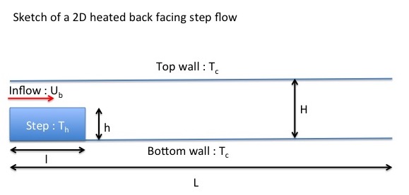
This tutorial shows how to create an input data file for a 2D heated back-facing step flow.
After providing the main features of the problem, explanations on how to build step by step the corresponding data file is shown.
Each relevant namelist is commented and referred to other pages for more details.
The user can create its own data file by resorting to any highlighted data set.
Flow characteristics
Description
The computation is on a 2D heated back-facing step flow. The temperature of the bottom and top walls is imposed to $T_c$ and the temperature of the step walls is $T_h$. The inflow is fixed with an uniform velocity profile $U_b$ at temperature $Tc$. We consider an incompressible flow under the Boussinesq hypothesis : the physical properties are constant and the thermal buoyancy effect is modelised by the Boussinesq hypothesis : $F_b= -\rho_0.\beta.g_0.(T - T_0)$ (see the page Gravity for more details). We suppose the fluid as a perfect gas. As a consequence, $\beta= \frac{1}{T_0}$
Dimensionless data
Reference scales for the dimensionless problem :
- the fluid density $\rho_0$
- the bulk velocity $U_b$
- the kinematic viscosity $\mu_0$
- the step height
- the temperature $T_c$
From the previous reference scales, we define the Reynolds number : $Re_h= \frac{\rho_0 \dot U_b \dot h}{\mu_0}$ and the dimensionless temperature $T*= \frac{T}{T_c}$.
We therefore deduce the following dimensionless data :
- Fluid density $\rho_0*=1$
- Inflow bulk velocity $U_b*= 1$
- Bottom and top wall temperature $T_c*=1$
- Thermal expansion coefficient $\beta*=1$
- Step height $h*= 1$
Any other data of the problem are set to :
- Domain length : $L*=12$
- Domain height : $H*= 2$
- Step length : $l*= 2$
- Reynolds number $Re_h= 100$
- Step wall temperature $T_h*= 2$
- Gravity constant $g*= \frac{g_0 \dot h}{U_b^2}= 1$
- Prandtl number $Pr= 0.71$
Data setup
We now build the data file by selecting the relevant namelists in the lookup list. We only keep the relevant variables (that must be explicitly set). The others ones are removed. We need to set :
Output data
Here we show an example of usual data acquisition :
- Instantaneous fields
- Statistical fields
- Time series from probes located at specific positions
The various parameters related to each type of output data are originally splitted by topic in the appropriate namelist. For a sake of clarity, they are directly regrouped for each type of output data as shown here :
For instantaneous fields
 &Field_Recording_Setup         Precision_On_Instantaneous_Fields= 2 /                  !--- option value for writing results in double precision (1 = single precision)
 &Simulation_Management         Fields_Recording_Rate = 1.0D-00 /                       !--- Recording rate (in time unit)
 &Instantaneous_Fields_Listing  Name_of_Field = "U" , Recording_Enabled = .true.  /     !--- Recording of the first velocity component enabled
 &Instantaneous_Fields_Listing  Name_of_Field = "V" , Recording_Enabled = .true.  /     !--- Recording of the second velocity component enabled
 &Instantaneous_Fields_Listing  Name_of_Field = "W" , Recording_Enabled = .false. /     !--- Recording of the Third velocity component disabled
 &Instantaneous_Fields_Listing  Name_of_Field = "T" , Recording_Enabled = .true.  /     !--- Recording Temperature enabled
 &Instantaneous_Fields_Listing  Name_of_Field = "P" , Recording_Enabled = .true.  /     !--- Recording Pressure enabled
For statistical fields
 &Simulation_Management Start_Time_For_Statistics= 1.D+2               ,          !--- Start time for computing the statistical fields
                        Time_Range_Statistic_Calculation = 1.D+00      /          !--- time range over which the statistical field computation is performed.
                                                                                        When it has been covered, the results are recorded and a new statistical computation starts again
 &Field_Recording_Setup      Precision_On_Statistical_Fields= 2 ,                 !--- option value for writing results in double precision (1 = single precision)
                             Time_Statistics_Enabled= .true.    ,                 !--- time statistics  are performed (true) - classical statistics (false)
                             Sample_Rate_For_Statistics= 1      ,                 !--- Sample rate (in time iteration unit)
                             Statistic_Space_Average_Type= "NO_SPACE_AVERAGE" /   !--- option on spatial averaged fields
 &Statistical_Fields_Listing  Name_of_Field = "<U>   " , Recording_Enabled = .true.  /   !---- Averaged I-velocity component
 &Statistical_Fields_Listing  Name_of_Field = "<V>   " , Recording_Enabled = .true.  /   !---- Averaged J-velocity component
 &Statistical_Fields_Listing  Name_of_Field = "<P>   " , Recording_Enabled = .true.  /   !---- Averaged pressure
For time-series from probes
                                                                       U    , V     , W      , T      , P     , RHO
 &Probe_Quantities_Enabled  Temporal_Series_For_Quantity_Enabled(:)= .true. , .true., .false., .false., .true., .false.    /    !--- Selection of physical quantities
 &Simulation_Management Probe_Recording_Rate                       = 10                                                     /   !--- Recording rate (in time-iteration unit)
 &Probe_Location  Xi= 2.0 , Xj= 1.5 , Xk= 0.0 /       !---coordinates of probe 1
 &Probe_Location  Xi= 3.0 , Xj= 1.0 , Xk= 0.0 /       !---coordinates of probe 2
- fr